Safety Stock
Safety stock is an inventory optimization method that indicates how much inventory need to be kept beyond the expected demand in order to achieve a given service level target. The extra stock acts as a “safety” buffer - hence the name - to protect the company against expected future fluctuations. The safety stock formula depends on both the expected future demand and the expected future lead time. The uncertainty is assumed to be normally distributed for both factors. The safety stock formula is ubiquitous is most inventory management systems, including most notable ERPs and MRPs.
Update July 2020: The approach detailed below is “textbook” supply chain, unfortunately, it also happens to be vastly dysfunctional. In particular, neither future demand not future lead time are normally distributed (i.e. not Gaussians). Moreover, the whole perspective entirely miss the point that all the SKUs that can be ordered or produced by the company compete for the same resources. We strongly advise not to use any safety stock model as far as real supply chains are concerned.
Intended audience: This document is primarily intended for supply chain professionals in retail or manufacturing. Yet, this document is also useful for accounting / ERP / eCommerce software editors that would like to extend their applications with stock management features.
We have tried to keep the mathematical requirements as low as possible, yet we can’t really avoid all formula altogether since the precise purpose of this document is to be a practical guide that explains how to compute safety stock.
Download: calculate-safety-stocks.xls (Microsoft Excel Spreadsheet)
Introduction
Inventory management is a financial trade-off between inventory costs and stock-out costs. The more stock, the more working capital is needed and the more stock depreciation you get. On the other hand if you do not have enough stock, you get inventory stock-outs, missing potential sales, possibility interrupting the whole production process.
Inventory stock depends essentially of two factors
- lead demand: the amount of items that will be consumed or bought.
- lead time: the delay between reorder decision and renewed availability.
Yet those two factors are subject to uncertainties
- demand variations: customer behaviors can evolve in rather unpredictable ways.
- lead time variations: suppliers or transporters may be faced with unplanned difficulties.
Deciding the level of safety stock is implicitly equivalent to making a trade-off between those costs considering the uncertainties.
The balance inventory costs vs. stock-outs costs is very business dependent. Thus, instead of considering those costs directly, we will now introduce the classical notion of service level.
The service level expresses the probability that a certain level of safety stock will not lead to stock-out. Naturally, when safety stocks are increased, the service level increases as well. When safety stocks get very large, the service level tends toward 100% (i.e. zero probability of encountering stock-out).
Choosing the service level, i.e. the acceptable probability of stock-out, is beyond the scope of this guide, but we have a separate guide about calculating optimal service levels.
Inventory replenishment model
The reorder point is the amount of stock that should trigger an order. If there was no uncertainty (i.e. future demand being perfectly known and supply being perfectly reliable), the reorder point would simply be equal to the total forecasted demand during the lead time, also called lead time demand.
In practice, because of the uncertainties, we have
reorder point = lead time demand + safety stock
If we assume that the forecasts are not biased (statistically speaking), having zero safety stocks would lead to a service level of 50%. Indeed, unbiased forecasts mean that there is as much chance for the future demand to be greater or lower than the lead time demand (remember that the lead time demand is just a forecasted value).
Caution: forecasts can be unbiased without being exact. The bias indicates a systematic error by the forecast model (ex: always over estimate the demand by 20%).
Normal distribution of the error
At this point, we need a way to represent the uncertainty in the lead time demand. In the following, we will assume that error is normally distributed, see the picture below.
Statistical notes: this normal distribution assumption is not totally arbitrary. Under certain situations, statistical estimators converge to a normal distribution as outlined by the Central limit theorem. But those considerations are beyond the scope of this guide.
A normal distribution is only defined by two parameters: its mean and its variance. Since we assume the forecasts to be unbiased, we assume the mean of the error distribution to be zero, which does not mean that we are assuming a zero error.
Determining the variance of the forecast error is a more delicate task. Lokad, as most forecasting toolkits, provides MAPE estimations (Mean Absolute Percentage Error) associated to its forecasts. For the sake of completeness, we will explain how simple heuristics can be used to overcome this problem.
In particular, the variance within the historical data can be used as a good heuristic to estimate the forecast error variance. David Piasecki also suggests to use the forecasted demand instead of the mean demand in the variance expression, that is
where $$E$$ is the mean operator, $$y_t$$ is the historical demand for the period $$t$$ (typically the amount of sales) and $$y’$$ the forecasted demand.
The key idea behind this assumption is that the forecast error is very often correlated to the amount of expected variation: the greater the upcoming variations, the greater the error in the forecasts.
Actually, the computation of this error variance involves a few subtleties that will be treated in greater details below.
Safety stock expression
At this point, we have determined both the mean and the variance, thus the error distribution is known. We must now calculate the acceptable error level within this distribution. Here above, we have introduced the notion of service level (a percentage) to do that.
Notes: We are assuming a static lead time. Yet, a very similar approach can be used for a varying lead time. See
In order to convert the service level into an error level also called the service factor, we must use the inverse cumulative normal distribution (sometimes also called inverse normal distribution) (see NORMSINV for the corresponding Excel function). As it might sounds complicated, it is not, we suggest to have a look at normal distribution applet to get a more visual insight. As you can see, the cumulative function transforms the percentage into an area-under-the-curve, the X axis threshold corresponding to the service factor value.
Intuitively, we calculate
safety stock = standard deviation of error * service factor
More formally, let $$S$$ be the safety stock, we have
where $$\sigma$$ is the standard deviation (i.e. the square root of $$\sigma^2$$ the variance defined here above), $$cdf$$ the normalized cumulative normal distribution (zero mean and variance equal to one) and $$P$$ the service level.
Remembering that
reorder point = lead time demand + safety stock
Let $$R$$ be the reorder point, we have
Matching lead time and forecast period
So far, we have been simply assuming that for a given lead time, we were directly able to produce the corresponding future demand forecast. In practice, it does not exactly work that way. The analysis of the historical data usually starts by aggregating the data into time periods (weeks or months typically).
Yet, the chosen period may not exactly match the lead time; thus, some further calculations are required to express the lead time demand and its associated variance (considering that we are still assuming a normal distribution for the forecast error, as detailed in the previous section).
Intuitively, the lead time demand can be computed as the sum of the forecasted values for the future periods that intersects the lead time segment. Care must be taken to properly adjust the last forecasted period.
Formally, let $$T$$ be the period and $$L$$ the lead time. We write
where $$k$$ integer and $$0 ≤ α < 1$$. Let $$D$$ be the lead time demand. Then, we have the final expression for the lead time demand
where $$y’_n$$ is the forecasted demand for the $$n^{th}$$ period in the future.
Considering the same normal distribution assumptions, we can compute the forecast error variance as
where $$y’$$ the average forecast per period
Yet, $$\sigma^2$$ is computed here as a per-period variance whereas we would need a variance that match the lead time instead. Let $$\sigma_{L}^2$$ be the adjusted per-lead-time variance, we have
Finally, we can re-express the reorder point as
Using Excel to compute the reorder point
This section details how to calculate the reorder point with Microsoft Excel. We suggest to have a look at the sample Excel spreadsheet provided.
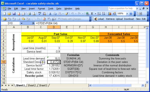
The sample sheet is basically split into two sections: the assumptions at the top and the calculations at the bottom. The forecasts are assumed to be part of the assumptions because sales (or demand) forecasting is beyond the scope of this guide. You can refer to our tutorial for sales forecasting with Microsoft Excel for details.
Most of the formulas introduced in the previous section are very plain operations (additions, multiplications) that are very easy to perform with Microsoft Excel. Yet, two functions are noticeable
- NORMSINV (Microsoft KB): estimates the cumulative normal distribution, noted cdf here above.
- STDEV (Microsoft KB): estimates standard deviation, noted $$σ$$ here above. We recall that the standard deviation $$σ$$ is the square root of the variance $${σ^2}$$.
For the sake of simplicity, the first sheet does not implement the heuristic $${σ^2 = E[ (y_t - y’)^2 ]}$$ when calculating the service factor. This approach is implemented in Sheet2 (2nd spreadsheet of the Excel document). Since we have assumed stationary forecasts in the example, the reorder point remains identical with or without this heuristic.
Resources
Inventory Management and Production Planning and Scheduling, Edward A. Silver, David F. Pyke, Rein Peterson, Wiley; 3 edition, 1998