Quantile Regression

By Joannès Vermorel, February 2012

The quantile regression a type of regression (i.e. forecast) that introduces on purpose a bias in the result. Instead of seeking the mean of the variable to be predicted, a quantile regression seeks the median and any other quantiles (sometimes named percentiles). Quantiles are particularly useful for inventory optimization as a direct method to compute the reorder point.

Regression is here a synomym for forecast. “Regression” emphasizes the mathematical approach, while “forecast” emphasizes the practical usage made of the result.

The notion of quantile regression is a relatively advance statistical topic, the goal of this article is not to go into a rigorous treatment of this subject, but rather to give a (relatively) intuitive introduction to the subject for practitioners in retail or manufacturing.

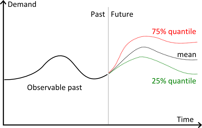
Visual illustration of quantiles

The lower and upper quantile time-series side-by-side with the mean forecast time-series.

The graph above illustrates 3 distinct forecasts:

in red, a 75% quantile forecasts.
in black, a mean forecast.
in green, a 25% quantile forecasts.

Visually, quantiles behaves pretty much like confidence intervals. However, in practice, the quantile is only needed for a single target percentage.

Quantiles (or percentiles) of future demand

The classical, and most intuitive, forecast is the mean forecast: the respective weights of over-forecasting and of under-forecasting should be equal, otherwise the forecast is biased (more precisely biased against the mean).

Although having a unbiased forecast is a desirable property, it does not tell anything about the accuracy of the forecast. In particular, a forecast can both unbiased yet widely inaccurate. The bias only refers to the propensity of the forecasting model to over or under estimate the future.

A first refinement of this vision is the median forecast: the respective frequency of over-forecasting and of under-forecasting should be equal, otherwise the forecasts is biased against the median.

At this point, we have already shifted the notion of unbiased forecasts from equal weights toward equal odds. This shift is subtle, but in some situations it might have be a big numerical impact.

Illustration: Mean vs Median household income in the US

The household income illustrates the profound difference between mean and median.

According to the US Census Bureau, in 2004, the median household income was $44,389 while the same year the mean (average) income was $60,528, nearly 40% higher than the median.

This discrepancy is explained by the high incomes (comparatively) of the richest US household compared to the rest of the population. Such discrepancy between mean and median will be found in all distributions that are not symmetric, typically all distributions that do not follow a normal distribution.

Generalization of the median

The median represents the threshold where the distribution is split on 50/50 odds. However, it is possible to consider other frequency ratios. For example, we can consider 80/20 or 90/10 or any other ratios where the total remains at 100%.

Quantiles represents a generalization of the median to any given percentage. For τ, a value between 0 and 1, the quantile regression Q(τ) represents the threshold where the probability of observing a value lower than the threshold is exactly τ.

Quantile forecasts

Both classic and quantile forecasts are taking a time-series as input. The time-series represent the input data. In addition to the data, a classic mean time-series forecasts requires two extra structural settings:

the period, such as day, week or month.
the horizon, an integer representing the number of periods to be forecast.

Implicitly, the time-series is aggregated according to the period, and the horizon is chosen as sufficiently large to be of practical use, typically greater than the lead time.

Mean forecasts benefit from a very handy property: it is mathematically correct to sum the forecasts. For example if y1, y2, y3 and y4 represent the 4 week ahead forecast, then if we need the expected demand only for the next two weeks, then we can sum y1+y2.

However, summing quantile forecasts is mathematically incorrect, or more precisely the sum of the quantiles does not yield the quantile of the sum (sum of the segments).

Let’s illustrate why quantile can’t be summed. Let’s a assume that we have a gambler playing one $1 coin into a slot machine each week. Let’s assume that the odds of winning are of 1% for a prize of $50 and zero otherwise. If we look at the 99% quantile of the expected reward, we have a weekly reward of $50 every week. However, if we look at the 99% quantile over two weeks, the expected reward is still equal to $50. Indeed, the probability of winning twice is only 0,01% (1% multiplied by 1%), hence the 99% quantile is left unchanged. Summing the two 99% weekly quantile would give $100, but in reality it takes 16 weeks to accumulate $100 of gain for the 99% quantile (the proof for this numerical result is not given as it would go beyond the scope of this article).

Since quantile forecasts cannot be summed, quantile time-series forecasts need to reconsider the very notion of period aggregation. Indeed, producing per period quantile forecasts is moot, because those elementary forecasts cannot be combined to produce correct quantiles over segments.

Thus, the quantile time-series forecast comes with a distinct structure:

τ the targeted quantile, a percentage.
λ the horizon expressing a duration (typically in days).

For example, if the time-series represent the sales of a product A, and we have the settings τ=0.90 and λ=14 days, then the quantile forecast (τ, λ) will return the demand value that has exactly 90% chance of being larger than the total demand observed over 14 days (respectively 10% chance of being lower than the demand over the same 14 days).

Contrary to classic forecasts, quantile forecasts are producing one and only one value per time-series, independently of the horizon. To a certain extent, quantile forecasts are more period-agnostic than their classic counterparts.

Lokad’s gotcha

At first glance, quantile forecasts look somewhat more complicated than the classic ones. Nevertheless, in many real-life situations, practitioners end-up producing first mean forecasts in order to extrapolate them immediately as quantile forecasts, typically assuming that the forecasts follow a normal distribution. However, this extrapolation step represents frequently the weakest link of the process, and may significantly degrade the final outcome. The forecasting technology should adapt to the practical requirements, i.e. delivering native quantile forecasts, and not the other way