ABC analysis (Inventory)
In inventory management, ABC analysis is an inventory categorization method used as a crude prioritization mechanism to concentrate efforts and resources on the items that matter the most for the company. This method is grounded in the empirical observation that a small fraction of the items or SKUs typically account for a large portion of the business. Before perpetual inventory systems became prevalent, ABC analysis was used to reduce the amount of clerical operations associated with inventory management. Since the 2000’s, this method is primarily used as a data visualization method, and as a way to prioritize the attention of supply chain practitioners, who have to routinely revisit replenishment settings within their inventory management system, such as Min/Max parameters or service levels.

Performing an ABC analysis
The ABC analysis is an inventory categorization method that assigns a class to every item - or SKU, or product - typically referred to as A, B and C, where A (resp. C) is the class associated with the most (resp. least) frequently sold or consumed items. There can be more than three classes (e.g. D, E, F, … ), although usually the number of classes is kept to a single digit count.
In order to compute the classes, the supply chain practitioner needs to choose a series of parameters that characterize the ABC analysis:
- the number of classes
- a unit to measure the “weight” of any item
- the historical depth of the measurement
- a percentage used as a threshold for each class.
The percentages are related to the unit chosen to measure the weight over the historical depth. Those percentages are typically related to the turnover measured in dollars or units sold.
While guidance can be provided in regards to the choice of those parameters, they fundamentally remain somewhat arbitrary. As the ABC analysis is intended to be accessible to a diverse audience within the company, parameters are usually chosen as round numbers that are easier to memorize.
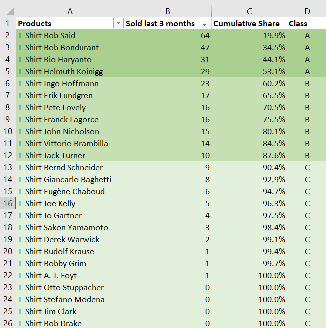
For example, the inventory manager of a niche ecommerce selling an assortment of 10,000 T-shirts for a yearly turnover of 50 million € decides to perform an ABC analysis with the following parameters:
- 3 classes (A, B, C)
- each unit sold counts as ‘1’
- the last 3 months of sales are considered
- the thresholds are 60% (A), 30% (B) and 10% (C).
Using a spreadsheet, the manager ranks in decreasing order all the items against their 3-months sales volumes - measured in units sold. Then, the thresholds are used against the cumulative share of the item weights. It is expected that the A class should have much fewer items than the C class. In the example below, the A/B/C classes have respectively 4/7/14 items.
Download the Excel spreadsheet: abc-analysis.xlsx
As illustrated with the Excel spreadsheet above, performing an ABC analysis is straightforward. Furthermore, many inventory softwares do feature ABC analysis - and frequently variants as well - as the implementation is a relatively trivial piece of software engineering.
The unit of measure can be eaches (i.e. units sold) if, as illustrated by the previous example, all items sold or serviced tend to have similar prices. However, if some items are considerably more expensive than others, then it typically makes more sense to weigh them against their purchase prices, or their selling prices.
The depth of history should be long enough for the averaged quantities to be statistically significant. Usually, classes are more stable if a multiple of common cyclicity is used, like one year, in order to neutralize the effect of seasonality, or an integral number of weeks to neutralize day-of-the-week effects when the depth is short.
The thresholds are typically adjusted so that each class has at least 5x more items than its predecessor. This ensures that a small number of classes covers even a large catalog. Starting with an A class of 100 items, and assuming 5x increments, the T-shirt retailer introduced above would need 4 classes to cover its entire catalog (100x5x5x5 = 12,500).
Pareto principle and power laws
The ABC analysis is based on the empirical observation, known as the Pareto principle or the 80/20 rule, that the top 20% of the items usually represent 80% of the sales volume, no matter which measurement unit is chosen. Thus, in such circumstances, it makes sense to segment the elements of interest - items in inventory - according to their “magnitude” of importance, i.e. the ABC classes.
From a more mathematical perspective, a magnitude-oriented analysis like ABC analysis is attractive whenever the underlying distribution (of probabilities) has a “fat tail”, i.e. points that are vastly diverging from the average1. Those situations happen frequently both in natural phenomena and human activities. For example, the following distributions are typically fat-tailed:
- company’s headcounts in a country
- biomass (in tons) of the species in an area
- box-office revenues of films for any given year
- recalls (in units) in the automotive industry
- …
There is a whole “bestiary” of mathematical distributions that are known to fit these situations. The most widely used distributions are probably the power law and the Zipf distribution. These mathematical functions mostly vary in their capacity to put “weight” on the tail of the distribution, i.e. in their capacity to reflect the odds of very rare situations occurring.
In the specific case of supply chains, simple economic forces are usually at play to artificially limit the magnitude of the outliers. For example, with back-to-inventory items, it can be remarked that the worst performers are typically removed from the assortment altogether. Thus, items which would sell, say, only once per year are not observed because the company stopped selling those items long before reaching this sales level.
Conversely, if an item is selling exceedingly well, then the company has an incentive to introduce variants - in color, size or any other technical attribute - in order to further increase its overall sales volume. Again, items which would sell tens of millions of units may never be observed, because by the time the item would have reached this volume, variants have been introduced that cannibalize the sales of the original item.
Common practices based on ABC analysis
The ABC analysis is used to support mundane inventory-related decisions, such as passing purchase orders to suppliers. While it is debatable whether practices based on ABC analysis can be considered as good practices (see section below on the limits of ABC analysis), certain practices are widespread such as:
- assigning service levels based on the class of items - the first classes have the highest targets, while the last classes have the lowest ones.
- assigning uniform manpower (attention) to every class - e.g. the supply chain practitioner spends 1 hour reviewing the A class (100 items), and then 1 hour reviewing the D class (10,000 items).
- segmenting all KPIs per class, and similarly segmenting all the dashboards or reports according to the class of interest. es- tablishing performance reviews - for supply chain teams - based on rules that depend on the ABC classes themselves.
Indeed, as the ABC classes are easy to produce and to maintain, these classes tend to blend themselves in with the company’s supply chain practices, as there is usually little resistance against what seems to be an intuitive way to refine an inventory-related analysis.
Historic materials management perspective
Historically, the ABC analysis emerged from a materials management perspective that was intended to minimize the clerical overheads associated with inventory. Each class of items would have its own specific set of processes:
- “A items” with very tight control and accurate records,
- “B items” with less tightly controlled and accurate records,
- “C items” with the simplest controls possible and minimal records.
Indeed, prior to the 70’s, inventory records had to be manually written in books by clercs, which was both slow and costly. Thus, in most situations, it was more efficient to adopt inventory management methods that did not require any record of any kind, like Kanban.
However, with the advent of low cost perpetual inventory systems and barcode readers, this practice has gradually faded away. Indeed, the risks associated with inventory movement lacking (digital) records, such as shrinkage, are now typically largely exceeding the clerical costs of maintaining those records. Thus, all items benefit from tight control and accurate records, i.e. the A item’s treatment, irrespective of their importance.
However, let’s point out that most companies still differentiate inventory - items being processed and sold - which need to be tracked - from general supplies (e.g. office supplies) which are not.
Intriguingly, many sources are still pointing to this historical perspective as the core motivation behind ABC analysis, while this practice has essentially disappeared from the processes of most mid and large companies since the early 2000’s.
The limits of ABC analysis
The ABC analysis is a crude inventory categorization method and exhibits many limitations. Those limits tend to exacerbate many pre-existing supply chain problems such as stockouts, overstocks, unreliability, and low productivity.
Instability. When using “reasonable” parameters, such as the ones given in the example above, ABC analysis frequently results in having between a quarter and a half of the items changing their category every quarter in numerous verticals. Worse, as assessing the stability of the ABC analysis is more complicated than performing the ABC analysis itself, most companies are not even aware of the problem. These instabilities put in jeopardy a large portion of the corrective measures, driven by the ABC classification, that end up being delivered to the wrong items.
Stationary-only. The ABC analysis is at odds with basic demand patterns like product launches: a newly introduced item has a low volume by design because its sales volume is yet to be observed. While it is possible to mitigate the novelty effect, other patterns, like seasonality, complicate the process. For example, in October, toys introduced 6 months before are classified as C items while Christmas sales are looming ahead. ABC analysis is a stationary perspective on the demand, and thus will generate inventory inefficiencies whenever the demand isn’t .
Low significance. As far as statistical indicators go, the amount of information extracted from the demand history and packed through the ABC classes is exceedingly low. For example, even a trivial indicator like “total units sold last year” tends to carry more information about any given item than its ABC class. Moreover, any statistical model performing any kind of task over the historical inventory data can internally re-implement an ABC analysis if it proves helpful - although, in practice, this is not the case.
Bikeshedding. The ABC analysis involves an arbitrary choice of parameters. As the ABC analysis has obvious shortcomings, like the product launches (see above), more parameters are usually introduced to mitigate those shortcomings. Then, as the ABC analysis is easy to grasp, a lot of people will invariably feel the need to be involved with the choice of all those parameters and/or request variants of their own. As a result, under the guise of a quick-and-easy method, the ABC analysis usually turns into a resource-consuming bureaucratic undertaking which does not deliver tangible results.
Blindness. Frequency does not equate with economic importance. The ABC analysis attributes importance of a product based on its frequency of usage or revenue. However, in many cases the unavailability of a not frequently consumed or valuable item can have the most devastating consequences and high stock levels and importance should be accorded to this item. An example from retail could be the merchandise effect where shiny items are placed in the window that are rarely sold yet crucial to attract customers. In manufacturing or aeronautics a specific part that may be used seldom and has little value from a purchase perspective may result in a commercial aircraft not being able to lift of.
Lokad’s take on ABC analysis
The ABC analysis was introduced early in the 20th century, in a world where barcode readers did not exist, and where inventory tracking methods were both expensive and unreliable. Surprisingly, this method has remained widespread while most of the problems that this method attempts to solve are long gone. Our general perspective on ABC analysis is the following: anything that the ABC analysis can do, even simpler methods perform better, like item scoring, rather than item classification. Naturally, all those simpler methods require computers to be executed, thus what can be considered as “simple” depends on the broader context to some extent.
For a purely reporting perspective, ABC analysis might be acceptable. ABC classes can help to gain rapid insights about product categories, for example, by reporting the respective fractions of A/B/C items within the category. However, as pointed out above, ABC analysis is prone to bikeshedding. Thus, we suggest to carefully avoid engineering indicators and KPIs on top of the A/B/C classes, as those initiatives nearly never deliver their originally intended benefits.
Notes
-
A fat-tailed distribution is a probability distribution that exhibits a large skewness or kurtosis, relative to that of either a normal distribution or an exponential distribution. Intuitively, it’s a distribution that does not follow the usual bell-shaped curve associated with, for example, the sizes (in cm) of the human population. ↩︎