Sparsity: when accuracy measure goes wrong
Three years ago, we were publishing Overfitting: when accuracy measure goes wrong, however overfitting is far from being the only situation where simple accuracy measurements can be very misleading. Today, we focus on a very error-prone situation: intermittent demand which is typically encountered when looking at sales at the store level (or Ecommerce).
We believe that this single problem alone has prevented most retailers to move toward advance forecasting systems at the store level. As with most forecasting problems, it’s subtle, it’s counterintuitive, and some companies charge a lot to bring poor answers to the question.

The most popular error metrics in sales forecasting are the Mean Absolute Error (MAE) and the Mean Absolute Percentage Error (MAPE). As a general guideline, we suggest to stick with the MAE as the MAPE behaves very poorly whenever time-series are not smooth, that is, all the time, as far retailers are concerned. However, there are situations where MAE too behaves poorly. Low sales volumes fall in those situations.
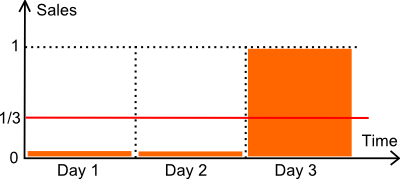
Let’s review the illustration here above. We have an item sold over 3 days. The number of unit sold over the first two days is zero. On the third day, one unit get sold. Let’s assume that the demand is, in fact, of exactly 1 unit every 3 days. Technically speaking, it’s a Poisson distribution with λ=1/3.
In the following, we compare two forecasting models:
- a flat model M at 1/3 every day (the mean).
- a flat model Z at zero every day.
As far inventory optmization is concerned, the model zero (Z) is downright harmfull. Assuming that safety stock analysis will be used to compute a reorder point, a zero forecast is very likely to produce a reorder point at zero too, causing frequent stockouts. An accuracy metric that would favor the model zero over more reasonable forecasts would be behaving rather poorly.
Let’s review our two models against the MAPE (*) and the MAE.
- M has a MAPE of 44%.
- Z has a MAPE of 33%.
- M has a MAE of 0.44.
- Z has a MAE of 0.33.
(*) The classic definition of MAPE involves a division by zero when the actual value is zero. We assume here that the actual value is replaced by 1 when at zero. Alternatively, we could also have divided by the forecast (instead of the actual value), or use the sMAPE. Those changes make no difference: the conclusion of the discussion remains the same.
In conclusion, here, according to both the MAPE and the MAE, model zero prevails.
However, one might argue that this is simplistic situation, and it does not reflect the complexity of a real store. This is not entirely true. We have performed benchmarks over dozens of retail stores, and usually the winning model (according to MAE or MAPE) is the model zero - the model that returns always zero. Futhermore, this model typically wins by a comfortable margin over all the other models.
In practice, at store level, relying either on MAE or MAPE to evaluate the quality of forecasting models is asking for trouble: the metric favors models that return zeroes; the more zeroes, the better. This conclusion holds for about every single store we have analyzed so far (minus the few high volume items that do not suffer this problem).
Readers who are familar with accuracy metrics might propose to go instead for the Mean Square Error (MSE) which will not favor the model zero. This is true, however, MSE when applied to erratic data - and sales are store level are erratic - is not numerically stable. In practice, any outlier in the sales history will vastly skew the final results. This sort of problem is THE reason why statisticians have been working so hard on robust statistics in the first place. No free lunch here.
How to assess store level forecasts then?
It took us a long, long time, to figure out a satifying solution to the problem of quantifying the accuracy of the forecasts at the store level. Back in 2011 and before, we were essentially cheating. Instead of looking at daily data points, when the sales data was too sparse, we were typically switching to weekly aggregates (or even to monthly aggregates for extremely sparse data). By switching to longer aggregation periods, we were artificially increasing sales volumes per period, hence making the MAE usable again.
The breakthrough came only a few months ago through quantiles. In essence, the enlightenment was: forget the forecasts, only reorder points matter. By trying to optimize our classic forecasts against metrics X, Y or Z, we were trying to solve the wrong problem.
Wait! Since reorder points are computed based on the forecasts, how could you say forecasts are irrelevant?
We are not saying that forecasts and forecast accuracy are irrelevant. However, we are stating that only the accuracy of the reorder points themselves matter. The forecast, or whatever other variable is used to compute reorder points, cannot be evaluated on its own. Only accuracy of the reorder points need and should be evaluated.
It turns out that a metric to assess reorder points exists: it’s the pinball loss function, a function that has been known by statisticians for decades. Pinball loss is vastly superior not because of its mathematical properties, but simply because it fits the inventory tradeoff: too much stocks vs too much stockouts.


