Generalization (Forecasting)
Generalization is the capacity of an algorithm to generate a model - leveraging a dataset - that performs well on previously unseen data. Generalization is of critical importance to supply chain, as most decisions reflect an anticipation of the future. In the forecasting context, the data is unseen because the model predicts future events, which are unobservable. While substantial progress, both theoretical and practical, has been achieved on the generalization front since the 1990s, true generalization remains elusive. The complete resolution of the generalization problem may not be very different from that of the artificial general intelligence problem. Furthermore, supply chain adds its own lot of thorny issues on top of the mainstream generalization challenges.

Overview of a paradox
Creating a model that performs perfectly on the data one has is straightforward: all it takes is to entirely memorize the dataset and then use the dataset itself to answer any query made about the dataset. As computers are good at recording large datasets, engineering such a model is easy. However, it is also usually pointless1, as the entire thrust of having a model lies in its predictive power beyond what has already been observed.
A seemingly ineluctable paradox presents itself: a good model is one that performs well on data that is currently unavailable but, by definition, if the data is unavailable, the observer cannot perform the assessment. The term “generalization”, therefore, refers to the elusive capability of certain models to retain their relevance and quality beyond the observations that are available at the time the model is constructed.
While memorizing the observations can be dismissed as an inadequate modelling strategy, any alternative strategy to create a model is potentially subject to the same problem. No matter how well the model appears to perform on data presently available, it is always conceivable that it is just a matter of chance, or worse, a defect of the modelling strategy. What may, at first, appear as a fringe statistical paradox is, in fact, a far-reaching issue.
By way of anecdotal evidence, in 1979 the SEC (Securities and Exchange Commission), the US agency in charge of regulating capital markets, introduced its famous Rule 156. This rule requires fund managers to inform investors that past performance is not indicative of future results. Past performance is implicitly the “model” that the SEC warns not to trust for its “generalization” power; that is, its ability to say anything about the future.
Even science itself is struggling with what it means to extrapolate “truth” outside a narrow set of observations. The “bad science” scandals, which unfolded in the 2000s and 2010s around p-hacking, indicate that entire fields of research are broken and cannot be trusted2. While there are cases of outright fraud where the experimental data has been plainly doctored, most of the time, the crux of the problem lies in the models; which is to say, in the intellectual process used to generalize what has been observed.
Under its most far-reaching guise, the generalization problem is indistinguishable from that of science itself, hence it is as difficult as replicating the breadth of human ingenuity and potential. Yet, the narrower statistical flavor of the generalization problem is much more approachable, and this is the perspective that will be adopted in the coming sections
Emergence of a new science
Generalization emerged as a statistical paradigm at the turn of the 20th century, primarily through the lens of forecasting accuracy3, which represents a special case tightly coupled to time-series forecasts. In the early 1900s, the emergence of a stock-owning middle class in the US generated massive interest in methods that would help people secure financial returns on their traded assets. Fortune tellers and economic forecasters alike deigned to extrapolate future events for an eagerly paying public. Fortunes were made and lost, but those efforts shed very little light on the “proper” way to approach the problem.
Generalization remained, by and large, a baffling problem for most of the 20th century. It was not even clear whether it belonged to the realm of natural sciences, governed by observations and experimentations, or to the realm of philosophy and mathematics, governed by logic and self-consistency.
The space trundled along until a landmark moment in 1982, the year of the first public forecasting competition - colloquially known as the M competition4. The principle was straightforward: publish a dataset of 1000 truncated time-series, let contenders submit their forecasts, and finally publish the rest of the dataset (the truncated tails) along with the respective accuracies achieved by the participants. Through this competition, generalization, still seen through the lens of forecasting accuracy, had entered the realm of natural sciences. Going forward, forecasting competitions became increasingly frequent.
A few decades later, Kaggle, founded in 2010, added a new dimension to such competitions by creating a platform dedicated to general prediction problems (not just time-series). As of February 20235, the platform has organized 349 competitions with cash prizes. The principle remains the same as the original M competition: a truncated dataset is made available, contenders submit their answers to the given prediction tasks, and finally, rankings along with the hidden portion of the dataset are revealed. The competitions are still considered the gold standard for the proper assessment of the generalization error of models.
Overfitting and underfitting
Overfitting, like its antonymous underfitting, is an issue that frequently arises while producing a model based on a given dataset, and undermines the generalization power of the model. Historically6, overfitting emerged as the first well-understood obstacle to generalization.
Visualizing overfitting can be done using a simple time-series modelling problem. For the purposes of this example, assume the aim is to create a model that reflects a series of historical observations. One of the simplest options to model these observations is a linear model as illustrated below (see Figure 1).
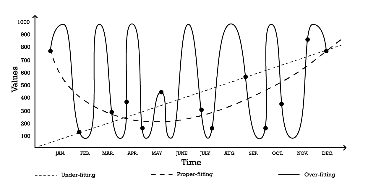
Figure 1: A composite graph depicting three different attempts at “fitting” a series of observations.
With two parameters, the “under-fitting” model is robust, but it, as the name suggests, underfits the data, as it clearly fails at capturing the overall shape of the distribution of observations. This linear approach has a high bias but a low variance. In this context, bias should be understood as the inherent limitation of the modeling strategy to capture the fine print of the observations, while variance should be understood as the sensitivity to small fluctuations – possibly noise – of the observations.
A fairly complex model could be adopted, as per the “over-fitting” curve (Figure 1). This model includes many parameters and exactly fits the observations. This approach has a low bias but a demonstrably high variance. Alternatively, a model of intermediate complexity could be adopted, as seen in the “proper-fitting” curve (Figure 1). This model includes three parameters, has a medium bias and a medium variance. Of these three options, the proper-fitting model is invariably the one that performs best as far as generalization is concerned.
These modeling options represent the essence of the bias-variance tradeoff.7 8 The bias-variance tradeoff is a general principle that outlines that the bias can be reduced by increasing the variance. The generalization error gets minimized by finding the proper balance between the amount of bias and variance.
Historically, from the early 20th century up to the early 2010s, an overfitted model was defined9 as one that contains more parameters than can be justified by the data. Indeed, at face value, adding too many degrees of freedom to a model appears to be the perfect recipe for overfitting issues. Yet, the emergence of deep learning proved this intuition, and the definition of overfitting, to be misleading. This point will be revisited in the section on deep double-descent.
Cross-validation and backtesting
Cross-validation is a model validation technique used to assess how well a model will generalize beyond its supporting dataset. It is a subsampling method that uses different portions of the data to respectively test and train a model on different iterations. Cross-validation is the bread and butter of modern prediction practices, and nearly all winning participants of prediction competitions make extensive use of cross-validation.
Numerous variants of cross-validation exist. The most popular variant is the k-fold validation where the original sample is randomly partitioned into k subsamples. Each subsample is used once as validation data, while the rest – all the other subsamples – is used as training data.
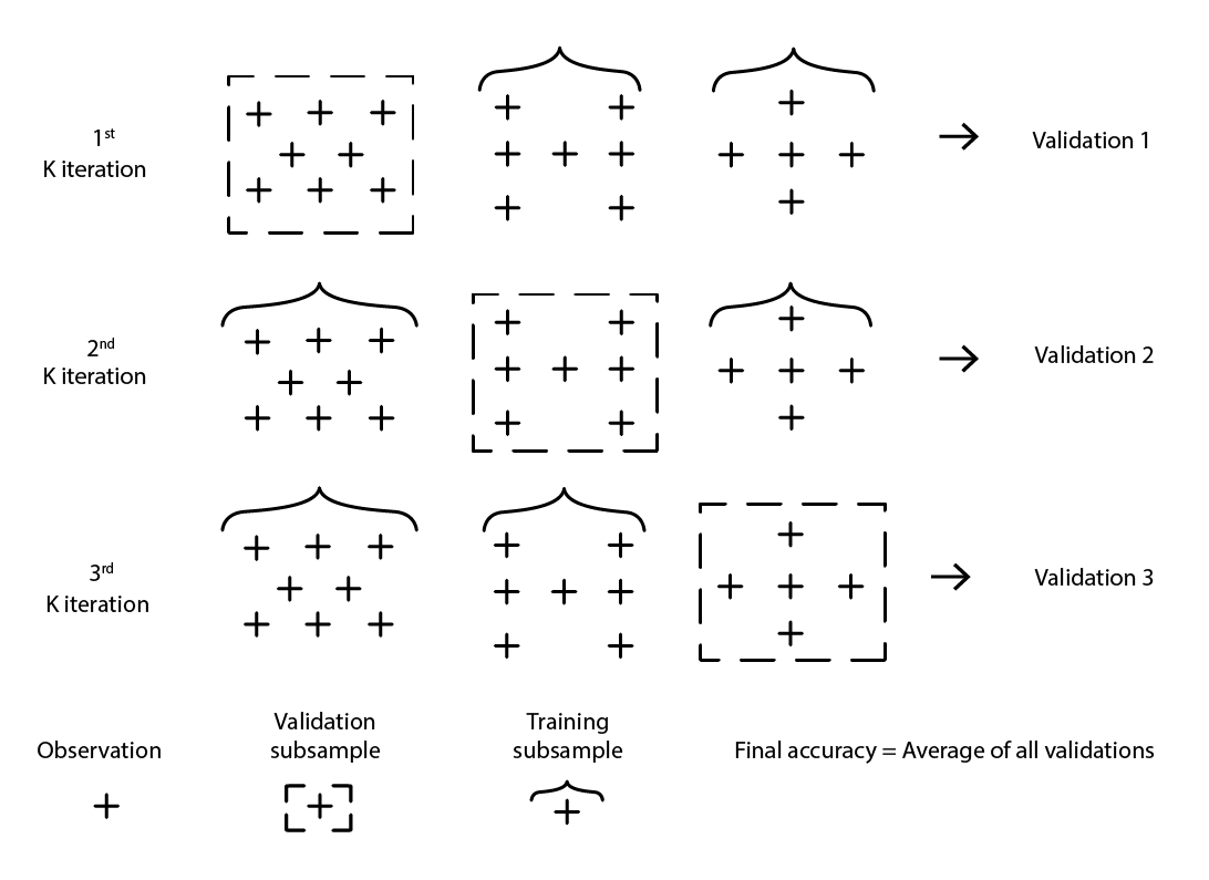
Figure 2: A sample K-fold validation. The observations above are all from the same dataset. The technique thus constructs data subsamples for validation and training purposes.
The choice of the value k, the number of subsamples, is a tradeoff between marginal statistical gains and the requirements in terms of computing resources. Indeed, with k-fold, the computing resources grow linearly with the value k while the benefits, in terms of error reduction, experience extreme diminishing returns10. In practice, selecting a value of 10 or 20 for k is usually “good enough”, as the statistical gains associated with higher values are not worth the extra inconvenience associated with the higher expenditure of computing resources.
Cross-validation assumes that the dataset can be decomposed into a series of independent observations. However, in supply chain, this is frequently not the case, as the dataset usually reflects some sort of historicized data where a time-dependence is present. In the presence of time, the training subsample must be enforced as strictly “preceding” the validation one. In other words, the “future”, relative to the resampling cutoff, must not leak into the validation subsample.
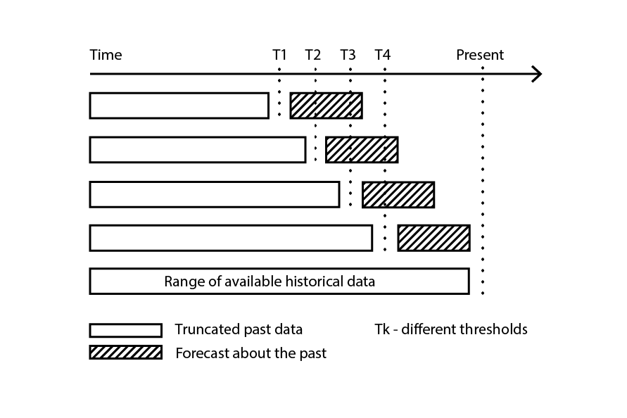
Figure 3: A sample backtesting process constructs data subsamples for validation and training purposes.
Backtesting represents the flavor of cross-validation that directly addresses the time-dependence. Instead of considering random subsamples, training and validation data are respectively obtained through a cutoff: observations prior to the cutoff belong to the training data, while observations posterior to the cutoff belong to the validation data. The process is iterated by picking a series of distinct cutoff values.
The resampling method that lies at the core of both cross-validation and backtesting is a powerful mechanism to steer the modeling effort towards a path of greater generalization. In fact, it is so efficient that there is an entire class of (machine) learning algorithms that embraces this very mechanism at their core. The most notable ones are random forests and gradient boosted trees.
Breaking the dimensional barrier
Quite naturally, the more data one has the more information there is to learn from. Hence, all things considered equal, more data should lead to better models, or at the very least, to models that are not any worse than their predecessors. After all, if more data makes the model worse, it is always possible to ignore the data as a last resort. Yet, due to overfitting problems, ditching data remained the lesser evil solution until the late 1990s. This was the crux of the “dimensional barrier” problem. This situation was both confounding and profoundly dissatisfying. Breakthroughs in the 1990s cracked the dimensional barriers with stunning insights, both theoretical and practical. In the process, those breakthroughs managed to derail – through sheer power of distraction – the entire field of study for a decade, delaying the advent of its successors, primarily deep learning methods - discussed in the next section.
To better grasp what used to be wrong with having more data, consider the following scenario: a fictitious manufacturer wants to predict the number of unscheduled repairs per year on large industrial pieces of equipment. After careful consideration of the problem, the engineering team has identified three independent factors that seem to contribute to the failure rates. However, the respective contribution of each factor in the overall failure rate is unclear.
Thus, a simple linear regression model with 3 input variables is introduced. The model can be written as Y = a1 * X1 + a2 * X2 + a3 * X3, where
- Y is the output of the linear model (the failure rate that the engineers want to predict)
- X1, X2 and X3 are the three factors (specific types of workloads expressed in hours of operation) that may contribute to the failures
- a1, a2 and a3 are the three model parameters that are to be identified.
The number of observations it takes to obtain “good enough” estimates for the three parameters is largely dependent on the level of noise present in the observation, and what qualifies as “good enough”. However, intuitively, to fit three parameters, two dozen observations would be required at minimum even in the most favorable situations. As the engineers are able to collect 100 observations, they successfully regress 3 parameters, and the resulting model appears “good enough” to be of practical interest. The model fails to capture many aspects of the 100 observations, making it a very rough approximation, but when this model is challenged against other situations through thought experiments, intuition and experience tell the engineers that the model seems to behave reasonably.
Based on their first success, the engineers decide to investigate deeper. This time, they leverage the full range of electronic sensors embedded in the machinery, and through the electronic records produced by those sensors, they manage to increase the set of input factors to 10,000. Initially, the dataset was comprised of 100 observations, with each observation characterized by 3 numbers. Now, the dataset has been expanded; it is still the same 100 observations, but there are 10,000 numbers per observation.
However, as the engineers try to apply the same approach to their vastly enriched dataset, the linear model does not work anymore. As there are 10,000 dimensions, the linear model comes with 10,000 parameters; and the 100 observations are nowhere near enough to support regressing that many parameters. The problem is not that it is impossible to find parameter values that fit, rather the exact opposite: it has become trivial to find endless sets of parameters that perfectly fit the observations. Yet, none of these “fitting” models are of any practical use. These “big” models perfectly fit the 100 observations, however, outside those observations, the models become nonsensical.
The engineers are confronted with the dimensional barrier: seemingly, the number of parameters must remain small compared to the observations, otherwise the modelling effort falls apart. This issue is vexing as the “bigger” dataset, with 10,000 dimensions rather than 3, is obviously more informative than the smaller one. Thus, a proper statistical model should be able to capture this extra information instead of becoming dysfunctional when confronted with it.
In the middle of the 1990s, a twofold breakthrough11, both theoretical and experimental, took the community by storm. The theoretical breakthrough was the Vapnik–Chervonenkis (VC) theory12. VC theory proved that, considering specific types of models, the real error could be upper bounded by what loosely amounted to the sum of the empirical error plus the structural risk, an intrinsic property of the model itself. In this context, “real error” is the error experienced on the data one does not have, while “empirical error” is the error experienced on the data one does have. By minimizing the sum of the empirical error and the structural risk, the real error could be minimized, as it was “boxed in”. This represented both a stunning result and arguably the biggest step towards generalization since the identification of the overfitting problem itself.
On the experimental front, models later known as Support Vector Machines (SVMs) were introduced almost as a textbook derivation of what VC theory had identified about learning. These SVMs became the first widely successful models capable of making satisfying use of datasets where the number of dimensions exceeded the number of observations.
By boxing the real error, a truly surprising theoretical result, VC theory had broken the dimensional barrier - something that had remained vexing for almost a century. It also paved the way for models capable of leveraging high dimensional data. Yet, soon enough, SVMs were themselves displaced by alternative models, primarily ensemble methods (random forests13 and gradient boosting), which proved in the early 2000s superior alternatives14, prevailing on both generalization and computing requirement fronts. Like the SVMs they replaced, ensemble methods also benefit from theoretical guarantees with regards to their capacity to avoid overfitting. All these methods shared the property of being non-parametric methods. The dimensional barrier had been broken through the introduction of models that did not need to introduce one or more parameters for every dimension; hence side-stepping a known path to overfitting woes.
Returning to the problem of unscheduled repairs mentioned earlier, unlike the classic statistical models – like linear regression, which falls apart against the dimensional barrier – ensemble methods would succeed in taking advantage of the large dataset and its 10,000 dimensions even though there are only 100 observations. What is more, ensemble methods would excel more or less out of the box. Operationally, this was quite a remarkable development, as it removed the need to meticulously craft models by picking the precisely correct set of input dimensions.
The impact on the broader community, both within and without academia, was massive. Most of the research efforts in the early 2000s were dedicated to exploring these nonparametric “theory-supported” approaches. Yet, successes evaporated rather quickly as the years passed. In fact, some twenty years on, the best models from what came to be known as the statistical learning perspective remain the same – merely benefiting from more performant implementations15.
The deep double-descent
Until 2010, conventional wisdom dictated that in order to avoid overfitting issues, the number of parameters had to remain much smaller than the number of observations. Indeed, as each parameter implicitly represented a degree of freedom, having as many parameters as observations was a recipe for ensuring overfitting16. Ensemble methods worked around the problem altogether by being nonparametric in the first place. Yet, this critical insight turned out to be wrong, and spectacularly so.
What came to be known later as the deep learning approach surprised almost the entire community through hyperparametric models. These are models that do not overfit yet contain many times more parameters than observations.
The genesis of deep learning is complex and can be traced back to the earliest attempts to model the processes of the brain, namely neural networks. Unpacking this genesis is beyond the scope of the present discussion, however, it is worth noting that the deep learning revolution of the early 2010s began just as the field abandoned the neural network metaphor in favor of mechanical sympathy. The deep learning implementations replaced the previous models with much simpler variants. These newer models took advantage of alternative computing hardware, notably GPUs (graphics processing units), which turned out to be, somewhat accidentally, well-suited for the linear algebra operations that characterize deep learning models17.
It took almost five more years for deep learning to be widely recognized as a breakthrough. A sizeable portion of the reticence came from the statistical learning camp - coincidentally, the section of the community that had successfully broken the dimensional barrier two decades earlier. While explanations vary for this reticence, the apparent contradiction between conventional overfitting wisdom and the deep learning claims certainly contributed to an appreciable level of initial skepticism regarding this newer class of models.
The contradiction remained largely unresolved until 2019, when the deep double descent was identified18, a phenomenon that characterizes the behavior of certain classes of models. For such models, increasing the number of parameters first degrades the test error (through overfitting), until the number of parameters becomes large enough to revert the trend and improve the test error again. The “second descent” (of the test error) was not a behavior predicted by the bias-tradeoff perspective.
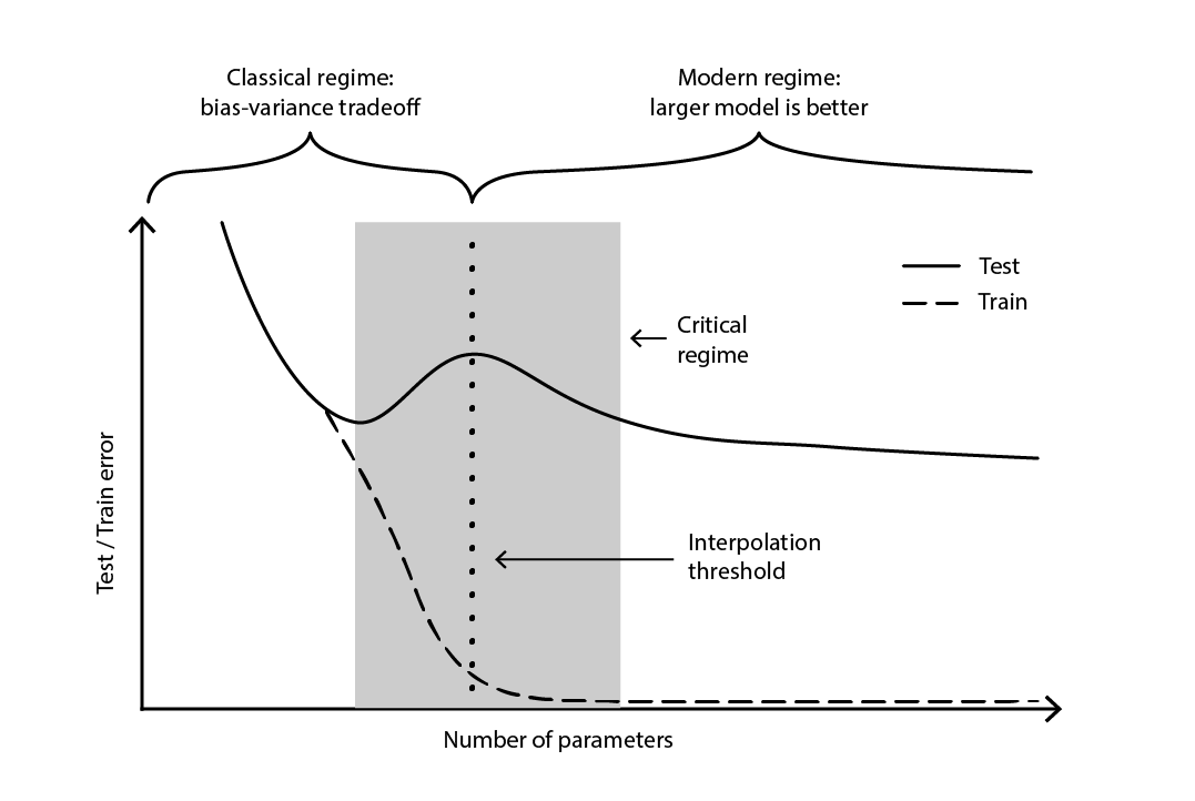
Figure 4. A deep double descent.
Figure 4 illustrates the two successive regimes described above. The first regime is the classic bias-variance tradeoff that seemingly comes with an “optimal” number of parameters. Yet, this minima turns out to be a local minima. There is a second regime, observable if one keeps increasing the number of parameters, that exhibits an asymptotic convergence towards an actual optimal test error for the model.
The deep double descent not only reconciled the statistical and deep learning perspectives, but also demonstrated that generalization remains relatively little understood. It proved that the widely-held theories – commonplace until the late 2010s - presented a distorted perspective on generalization. However, the deep double descent does not yet provide a framework – or something equivalent – that would predict the generalization powers (or lack thereof) of models based on their structure. To date, the approach remains resolutely empirical.
The supply chain thorns
As covered in depth, generalization is exceedingly challenging, and supply chains manage to throw in their own lot of quirks, further intensifying the situation. First, the data supply chain practitioners seek may forever remain inaccessible; not fractionally unseen, but wholly unobservable. Second, the very act of prediction may alter the future, and the validity of the prediction, as decisions are built upon those very predictions. Thus, when approaching generalization in a supply chain context, a two-legged approach should be used; one leg being the statistical soundness of the model and the other being the high-level reasoning that supports the model.
Furthermore, the available data is not always the desired data. Consider a manufacturer that wants to forecast demand in order to decide the quantities to be produced. There is no such thing as historical “demand” data. Instead, the historical sales data represents the best proxy available to the manufacturer to reflect historical demand. However, historical sales are distorted by past stock-outs. Zero sales, as caused by stock-outs, should not be confused with zero demand. While a model can be crafted to rectify this sales history into some sort of demand history, the generalization error of this model is elusive by design, as neither the past nor the future holds this data. In short, “demand” is a necessary but intangible construct.
In machine learning jargon, modeling demand is an unsupervised learning problem where the output of the model is never observed directly. This unsupervised aspect defeats most learning algorithms, and most model validation techniques as well – at least, in their “naïve” flavor. Moreover, it also defeats the very idea of prediction competition, here meaning a simple two-stage process where an original dataset is split into a public (training) subset and a private (validation) subset. The validation itself becomes a modelling exercise, by necessity.
Simply put, the prediction created by the manufacturer will shape, one way or another, the future the manufacturer experiences. A high projected demand means that the manufacturer will ramp up production. If the business is well-run, economies of scale are likely to be achieved in the manufacturing process, hence lowering production costs. In turn, the manufacturer is likely to take advantage of these newfound economics in order to lower prices, hence gaining a competitive edge over rivals. The market, seeking the lowest priced option, may swiftly adopt this manufacturer as its most competitive option, hence triggering a surge of demand well beyond the initial projection.
This phenomenon is known as a self-fulfilling prophecy, a prediction that tends to become true by virtue of the influencing belief that the participants have in the prediction itself. An unorthodox, but not entirely unreasonable, perspective would characterize supply chains as giant self-fulfilling Rube Goldberg contraptions. At a methodological level, this entanglement of observer and observation further complicates the situation, as generalization becomes associated with the capture of the strategic intent that underlies the supply chain developments.
At this point, the generalization challenge, as it presents itself in supply chain, might appear insurmountable. Spreadsheets, which remain ubiquitous in supply chains, certainly hint that this is the default, albeit implicit, position of most companies. A spreadsheet is, however, first and foremost a tool for deferring the resolution of the problem to some ad-hoc human judgement, rather than the application of any systematic method.
Though deferring to human judgement is invariably the incorrect response (in and of itself), it is not a satisfying answer to the problem, either. The presence of stock-outs does not mean that anything goes as far as demand is concerned. Certainly, if the manufacturer has maintained average service levels above 90% during the last three years, it would be highly improbable that (observed) demand could have been 10 times more than sales. Thus, it is reasonable to expect that a systematic method can be engineered to cope with such distortions. Similarly, the self-fulfilling prophecy can be modeled as well, most notably through the notion of policy as understood by the control theory.
Thus, when considering a real-world supply chain, generalization requires a two-legged approach. First, the model must be statistically sound, to the extent permitted by the broad “learning” sciences. This encompasses not only theoretical perspectives like classical statistics and statistical learning, but also empirical endeavors like machine learning and prediction competitions. Reverting to 19th century statistics is not a reasonable proposition for a 21st century supply chain practice.
Second, the model must be supported by high-level reasoning. In other words, for every component of the model and every step of the modeling process, there should be a justification that makes sense from a supply chain perspective. Without this ingredient, operational chaos19 is almost guaranteed, usually triggered by some evolution of the supply chain itself, its operating ecosystem, or its underlying applicative landscape. Indeed, the whole point of high-level reasoning is not to make some model work once, rather to make it work sustainably across several years in an ever-changing environment. This reasoning is the not-so-secret ingredient that helps decide it is time to revise the model when its design, whatever it is, no longer aligns with reality and/or business goals.
From afar, this proposition might seem vulnerable to the earlier critique addressed to spreadsheets – the one against deferring hard work to some elusive “human judgement”. Though this proposition still defers the assessment of the model to human judgement, the execution of the model is intended as fully automated. Thus, daily operations are intended to be fully automated, even if the ongoing engineering efforts to improve further the numerical recipes are not.
Notes
-
There is an important algorithmic technique called “memoization" that precisely replaces a result thatby could be recomputed by its pre-computed result, hence trading more memory for less compute. However, this technique is not relevant to the present discussion. ↩︎
-
Why Most Published Research Findings Are False, John P. A. Ioannidis, August 2005 ↩︎
-
From the time-series forecasting perspective, the notion of generalization is approached via the concept of “accuracy”. Accuracy can be seen as a special case of “generalization” when considering time-series. ↩︎
-
Makridakis, S.; Andersen, A.; Carbone, R.; Fildes, R.; Hibon, M.; Lewandowski, R.; Newton, J.; Parzen, E.; Winkler, R. (April 1982). “The accuracy of extrapolation (time series) methods: Results of a forecasting competition”. Journal of Forecasting. 1 (2): 111–153. doi:10.1002/for.3980010202. ↩︎
-
Kaggle in Numbers, Carl McBride Ellis, retrieved February 8th 2023, ↩︎
-
The 1935 excerpt “Perhaps we are old fashioned but to us a six-variate analysis based on thirteen observations seems rather like overfitting”, from “The Quarterly Review of Biology” (Sep, 1935 Volume 10, Number 3pp. 341 – 377), seems to indicate that the statistical concept of overfitting was already established by that time. ↩︎
-
Grenander, Ulf. On empirical spectral analysis of stochastic processes. Ark. Mat., 1(6):503– 531, 08 1952. ↩︎
-
Whittle, P. Tests of Fit in Time Series, Vol. 39, No. 3/4 (Dec., 1952), pp. 309-318] (10 pages), Oxford University Press ↩︎
-
Everitt B.S., Skrondal A. (2010), Cambridge Dictionary of Statistics, Cambridge University Press. ↩︎
-
The asymptotical benefits of using greater k values for the k-fold can be inferred from the central limit theorem. This insight hints that, by increasing k, we can get approximately 1 / sqrt(k) close from exhausting the entire improvement potential brought by the k fold in the first place. ↩︎
-
Support-vector networks, Corinna Cortes, Vladimir Vapnik, Machine Learning volume 20, pages 273–297 (1995) ↩︎
-
The Vapnik-Chernovenkis (VC) theory was not the only candidate to formalize what “learning” means. Valiant’s 1984 PAC (probably approximately correct) framework paved the way for formal learning approaches. However, the PAC framework lacked the immense traction, and the operational successes, that the VC theory enjoyed around the millennium. ↩︎
-
Random Forests, Leo Breiman, Machine Learning volume 45, pages 5–32 (2001) ↩︎
-
One of the unfortunate consequences of Support Vector Machines (SVMs) being heavily inspired by a mathematical theory is that those models have little “mechanical sympathy” for modern computing hardware. The relative inadequacy of SVMs to process large datasets – including millions of observations or more – compared to alternatives spelled the downfall of those methods. ↩︎
-
XGBoost and LightGBM are two open-source implementations of the ensemble methods that remain widely popular within machine learning circles. ↩︎
-
For the sake of concision, there is a bit of oversimplification going on here. There is an entire field of research dedicated to the “regularization” of statistical models. In the presence of regularization constraints, the number of parameters, even considering a classic model like a linear regression, may safely exceed the number of observations. In the presence of regularization, no parameter value quite represents a full degree of freedom anymore, rather a fraction of one. Thus, it would be more proper to refer to the number of degrees of freedom, instead of referring to the number of parameters. As these tangential considerations do not fundamentally alter the views presented here, the simplified version will suffice. ↩︎
-
In fact, the causality is the other way around. Deep learning pioneers managed to re-engineer their original models - neural networks - into simpler models that relied almost exclusively on linear algebra. The point of this re-engineering was precisely to make it possible to run these newer models on computing hardware that traded versatility for raw power, namely GPUs. ↩︎
-
Deep Double Descent: Where Bigger Models and More Data Hurt, Preetum Nakkiran, Gal Kaplun, Yamini Bansal, Tristan Yang, Boaz Barak, Ilya Sutskever, December 2019 ↩︎
-
The vast majority of the data science initiatives in supply chain fail. My casual observations indicate that the data scientist’s ignorance of what makes the supply chain tick is the root cause of most of these failures. Although it is incredibly tempting – for a newly trained data scientist - to leverage the latest and shiniest open-source machine learning package, not all modeling techniques are equally suited to support high-level reasoning. In fact, most of the “mainstream” techniques are downright terrible when it comes to the whiteboxing process. ↩︎