一般化 (予測)
一般化とは、アルゴリズムがデータセットを活用して、これまで見たことのないデータに対しても優れた性能を発揮するモデルを生成する能力を指します。一般化はサプライチェーンにとって極めて重要であり、ほとんどの意思決定が将来の予測に基づいて行われるためです。予測の文脈において、データが見えない理由は、モデルが観察不可能な未来の出来事を予測するためです。1990年代以降、理論的にも実用的にも大きな進歩があったにもかかわらず、本当の意味での一般化は未だ捉えがたいものです。一般化問題の完全な解決は、人工汎用知能問題の解決と大差ないかもしれません。さらに、サプライチェーンは主流の一般化の課題に加えて、独自の厄介な問題を多く抱えています。

パラドックスの概要
手元にあるデータに対して完璧に機能するモデルを作成することは簡単です:必要なのは、データセットを完全に記憶し、そのデータセット自体を用いてデータセットに関するあらゆる問いに答えることです。コンピューターは大規模なデータセットの記録が得意なため、そのようなモデルを構築するのは容易です。しかし、これは通常、無意味です1。というのも、モデルを持つ本来の目的は、すでに観測されたものを超えた予測力にあるからです。
一見避けがたいパラドックスが現れます:良いモデルとは、現在利用できないデータに対してもうまく機能するモデルであるということですが、定義上、データが利用できない場合、評価を行うことはできません。従って、「一般化」という用語は、モデル構築時に存在する観測を超えて、その関連性と質を維持するモデルの捉えがたい能力を指します。
観測値を単に記憶することは不十分なモデリング戦略として却下されるかもしれませんが、モデルを作成するための他のいかなる戦略も同様の問題に直面する可能性があります。現在利用可能なデータに対してモデルが優れているように見えても、それが単なる偶然の産物であるか、さらにはモデリング戦略の欠陥によるものである可能性は常に否定できません。一見、周辺的な統計上のパラドックスに思える問題は、実際には極めて広範な問題なのです。
逸話的な証拠として、1979年に米国の資本市場を規制する機関であるSEC(証券取引委員会)は、有名な Rule 156 を導入しました。この規則は、ファンドマネージャーに対して、過去の実績が将来の結果を保証するものではない ことを投資家に知らせることを義務付けています。過去の実績は、SECがその「一般化」能力、すなわち将来について何かを語る力に対して信頼すべきでないと警告する「モデル」と暗黙のうちに見なされているのです。
科学そのものですら、狭い観測範囲の外に「真実」を外挿することの意味に苦戦しています。2000年代や2010年代に明るみに出た p-hacking 周辺の「悪い科学」スキャンダルは、研究分野全体が壊れており、信用できないことを示しています2。実験データが明らかに改ざんされた明白な詐欺事例もありますが、ほとんどの場合、問題の核心は観測されたものを 一般化 するために用いられた知的プロセス、つまり、モデルそのものにあります。
最も大局的な姿では、一般化の問題は科学そのものの問題と見分けがつかなくなるため、人間の創造力と可能性の広がりを再現するのと同じくらい難解です。しかし、一般化問題のより狭義の統計的側面ははるかに理解しやすく、以降のセクションではこの観点から議論を進めていきます。
新たな科学の出現
一般化は20世紀初頭に 予測精度3 の視点から、統計パラダイムとして登場しました。これは、時系列予測に密接に結びついた特殊なケースを表しています。1900年代初頭、米国で株式を保有する中産階級が台頭する中、人々が取引資産から金融リターンを確保するための方法に対して大きな関心が寄せられました。占い師や経済予測士は、熱心に支払う大衆のために未来の出来事を外挿することに挑みました。結果として富は生み出され、また失われましたが、これらの試みは問題に対する「適切な」アプローチ方法についてほとんど光を当てませんでした。
一般化は、20世紀の大部分において、ほとんどの人にとって理解し難い問題として残りました。それが、観測と実験に支配される自然科学の領域に属するのか、それとも論理と一貫性によって支配される哲学や数学の領域に属するのか、明確ではなかったのです。
物事は進み、1982年、最初の公開予測コンペティション、通称 M コンペティション4という画期的な瞬間を迎えました。原則は単純でした:1000本の短縮時系列のデータセットを公開し、参加者に予測を提出させ、最後に残りのデータ(短縮された部分)と各参加者の達成した精度を公開するというものでした。このコンペティションを通じて、依然として 予測精度 の視点から見られていた一般化は、自然科学の領域に足を踏み入れました。以降、予測コンペティションはますます頻繁に開催されるようになりました。
数十年後、2010年に設立された Kaggle は、時系列に限らない一般的な予測問題に特化したプラットフォームを作ることで、こうしたコンペティションに新たな次元を加えました。2023年2月現在5、このプラットフォームは賞金付きで349回のコンペティションを開催しています。その原則は当初の M コンペティションと同じで、短縮データセットが提供され、参加者が与えられた予測タスクに対する回答を提出し、最後にランキングと隠されたデータの一部が明らかにされるというものです。これらのコンペティションは、モデルの一般化誤差を適切に評価するためのゴールドスタンダードと見なされています。
過学習と低学習
過学習(反意語である 低学習 と同様に)は、与えられたデータセットに基づいてモデルを作成する際によく発生する問題で、モデルの一般化能力を損ないます。歴史的には6、過学習は一般化に対する最初のよく理解された障害として浮上しました。
シンプルな時系列モデリングの問題を用いて 過学習 を視覚化することができます。この例のために、目的は一連の過去の観測値を反映するモデルを作成することだと仮定します。これらの観測値をモデル化する最も簡単なオプションの一つは、以下に示すような線形モデルです(Figure 1参照)。
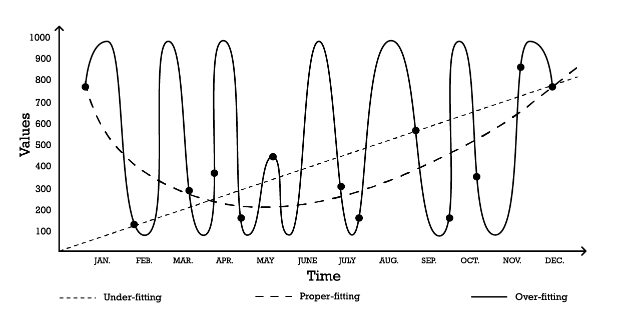
Figure 1: 一連の観測値に対して「フィッティング」を試みた3つの異なる試みを示す合成グラフ
2つのパラメータを持つ「低学習」モデルは安定していますが、その名が示す通り、データの全体的な分布の形状を捉えきれていません。この線形アプローチはバイアスが高く、分散が低いのが特徴です。この文脈では、バイアス は観測値の詳細を捉えるためのモデリング戦略の固有の限界として理解されるべきであり、分散 は観測値の小さな変動、すなわちノイズに対する感受性として理解されるべきです。
「過学習」曲線(Figure 1)に示されるように、かなり複雑なモデルを採用することも可能です。このモデルは多くのパラメータを含み、観測値に正確にフィットします。このアプローチはバイアスが低いものの、明らかに分散が高いです。あるいは、中程度の複雑さを持つモデル、いわゆる「適切なフィッティング」モデル(Figure 1参照)を採用することもできます。このモデルは3つのパラメータを含み、バイアスも分散も中程度です。これら3つのオプションの中で、一般化に関しては常に 適切なフィッティング モデルが最も良い性能を発揮します。
これらのモデリングオプションは、バイアスと分散のトレードオフの本質を表しています7。8 バイアスは分散を増加させることで減少できると概説されており、一般化誤差はバイアスと分散の適切なバランスを見つけることによって最小化されます。
歴史的には、20世紀初頭から2010年代初頭にかけて、過学習モデルは9 データによって正当化される以上のパラメータを含むものとして定義されていました。実際、表面的には、モデルに自由度を加えすぎることは過学習問題の完璧なレシピのように見えます。しかし、ディープラーニングの登場はこの直感、そして過学習の定義を誤解を招くものとしていることを証明しました。この点はディープ・ダブル・ディセントのセクションで改めて論じられます。
クロスバリデーションとバックテスト
クロスバリデーションは、モデルがサポートデータセットを超えてどれだけ一般化できるかを評価するためのモデル検証手法です。これは、異なる部分のデータを用いて、交互にモデルのテストとトレーニングを行うサブサンプリング手法です。クロスバリデーションは現代の予測手法の基本であり、予測コンペティションのほぼ全ての勝者が広範に利用しています。
クロスバリデーションには多くのバリエーションがあります。最も一般的なバリエーションは k 分割検証で、元のサンプルをランダムに k 個のサブサンプルに分割します。各サブサンプルは一度だけ検証データとして使用され、残りのサブサンプルはすべて トレーニングデータ として使用されます。
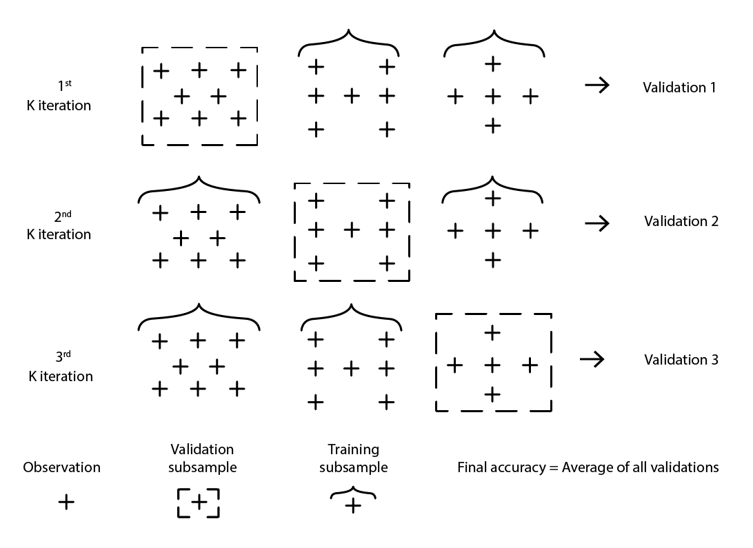
Figure 2: 同一のデータセットからの観測値を用いたサンプルのK-分割検証。 この手法により、検証とトレーニングのためのデータサブサンプルが構築されます。
k、つまりサブサンプルの数の選択は、統計的な利益と計算資源の要求との間のトレードオフです。実際、k 分割検証では計算資源は k に応じて線形に増加する一方、誤差削減という観点からの利益は著しく逓減します10。実務上、k の値を10または20に設定することが通常「十分良好」とされ、高い値による統計的利益は、計算資源の余分な消費による不便さに見合うものではありません。
クロスバリデーションは、データセットが一連の独立した観測値に分解できることを前提としています。しかし、サプライチェーンにおいては、データセットは通常、時系列依存性を伴う過去のデータを反映しているため、その前提は必ずしも成り立ちません。時間が存在する場合、トレーニング用のサブサンプルは検証用サブサンプルよりも厳密に「先行」している必要があります。言い換えれば、再サンプリングのカットオフに対して「未来」が検証用サブサンプルに流入してはいけないのです。
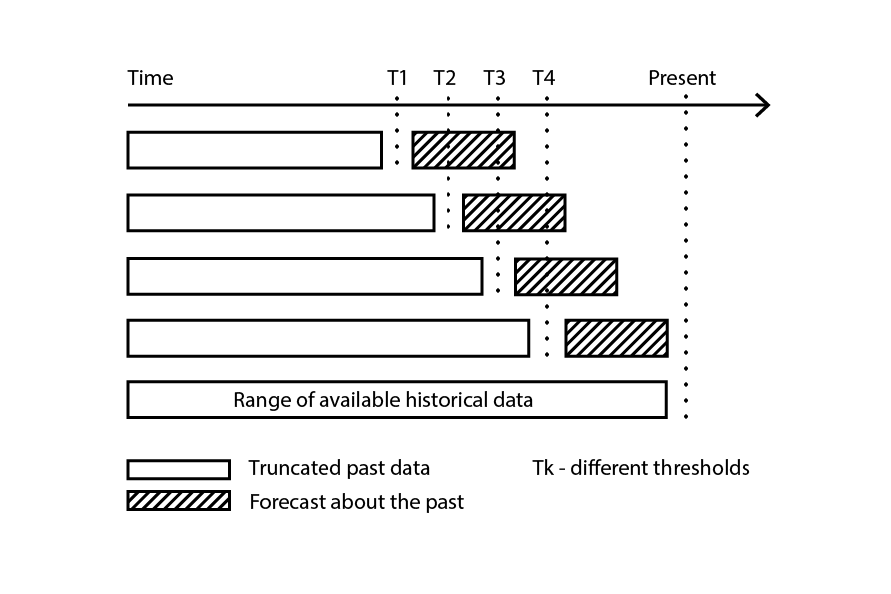
Figure 3: データのサブサンプルを検証とトレーニングの目的で構築するバックテストのプロセスの例。
バックテスト は、時系列依存性に直接対応するクロスバリデーションの一形態です。ランダムなサブサンプルを考慮する代わりに、トレーニングデータと検証データはそれぞれカットオフによって取得され、カットオフより前の観測値はトレーニングデータに、カットオフ以降の観測値は検証データに属します。このプロセスは、異なるカットオフ値の一連を選択することで繰り返されます。
クロスバリデーションとバックテストの両方の核心にある再サンプリング手法は、モデリング努力をより高い一般化へと導く強力なメカニズムです。実際、この手法を中核とする(機械)学習アルゴリズムのクラスが存在するほど、その効率性は高いです。最も顕著なものは、ランダムフォレストや勾配ブースト木です。
次元の壁を打破する
当然ながら、データが多ければ多いほど、学ぶべき情報も増えます。したがって、他の条件が同じであれば、より多くのデータはより良いモデル、あるいは少なくともそれまでのモデルより悪くないモデルにつながるはずです。結局のところ、データが多くなることでモデルが悪化する場合は、最終手段としてデータを無視することも可能です。しかし、過学習の問題があるため、1990年代後半まではデータを削減することが より小さい悪 として残っていました。これが「次元の壁」問題の核心でした。この状況は困惑させると同時に、非常に不満をもたらすものでした。1990年代の突破口は、理論的にも実践的にも驚くべき洞察をもたらし、次元の壁を打破しました。その過程で、これらの突破口は大きな話題をさらい、この分野全体の進展を10年間遅らせ、主に次のセクションで議論されるディープラーニング手法の登場を遅らせました。
より多くのデータを持つことにかつてどのような問題があったのかをよりよく理解するために、以下のシナリオを考えてみましょう:ある架空のメーカーが、大型産業用機器の年間の計画外修理件数を予測したいとします。
そこで、3つの入力変数を持つ単純な線形回帰モデルが導入されます。このモデルは Y = a1 * X1 + a2 * X2 + a3 * X3 と記述することができます。ここで
-
Y は線形モデルの出力(エンジニアが予測したい故障率)です。
-
X1, X2, および X3 は、故障に寄与する可能性のある3つの要因(稼働時間で表現される特定の作業負荷の種類)です。
The number of observations it takes to obtain “good enough” estimates for the three parameters is largely dependent on the level of noise present in the observation, and what qualifies as “good enough”. However, intuitively, to fit three parameters, two dozen observations would be required at minimum even in the most favorable situations. As the engineers are able to collect 100 observations, they successfully regress 3 parameters, and the resulting model appears “good enough” to be of practical interest. The model fails to capture many aspects of the 100 observations, making it a very rough approximation, but when this model is challenged against other situations through thought experiments, intuition and experience tell the engineers that the model seems to behave reasonably.
Based on their first success, the engineers decide to investigate deeper. This time, they leverage the full range of electronic sensors embedded in the machinery, and through the electronic records produced by those sensors, they manage to increase the set of input factors to 10,000. Initially, the dataset was comprised of 100 observations, with each observation characterized by 3 numbers. Now, the dataset has been expanded; it is still the same 100 observations, but there are 10,000 numbers per observation.
However, as the engineers try to apply the same approach to their vastly enriched dataset, the linear model does not work anymore. As there are 10,000 dimensions, the linear model comes with 10,000 parameters; and the 100 observations are nowhere near enough to support regressing that many parameters. The problem is not that it is impossible to find parameter values that fit, rather the exact opposite: it has become trivial to find endless sets of parameters that perfectly fit the observations. Yet, none of these “fitting” models are of any practical use. These “big” models perfectly fit the 100 observations, however, outside those observations, the models become nonsensical.
The engineers are confronted with the dimensional barrier: seemingly, the number of parameters must remain small compared to the observations, otherwise the modelling effort falls apart. This issue is vexing as the “bigger” dataset, with 10,000 dimensions rather than 3, is obviously more informative than the smaller one. Thus, a proper statistical model should be able to capture this extra information instead of becoming dysfunctional when confronted with it.
In the middle of the 1990s, a twofold breakthrough11, both theoretical and experimental, took the community by storm. The theoretical breakthrough was the Vapnik–Chervonenkis (VC) theory12. VC theory proved that, considering specific types of models, the real error could be upper bounded by what loosely amounted to the sum of the empirical error plus the structural risk, an intrinsic property of the model itself. In this context, “real error” is the error experienced on the data one does not have, while “empirical error” is the error experienced on the data one does have. By minimizing the sum of the empirical error and the structural risk, the real error could be minimized, as it was “boxed in”. This represented both a stunning result and arguably the biggest step towards generalization since the identification of the overfitting problem itself.
On the experimental front, models later known as Support Vector Machines (SVMs) were introduced almost as a textbook derivation of what VC theory had identified about learning. These SVMs became the first widely successful models capable of making satisfying use of datasets where the number of dimensions exceeded the number of observations.
By boxing the real error, a truly surprising theoretical result, VC theory had broken the dimensional barrier - something that had remained vexing for almost a century. It also paved the way for models capable of leveraging high dimensional data. Yet, soon enough, SVMs were themselves displaced by alternative models, primarily ensemble methods (random forests13 and gradient boosting), which proved in the early 2000s superior alternatives14, prevailing on both generalization and computing requirement fronts. Like the SVMs they replaced, ensemble methods also benefit from theoretical guarantees with regards to their capacity to avoid overfitting. All these methods shared the property of being non-parametric methods. The dimensional barrier had been broken through the introduction of models that did not need to introduce one or more parameters for every dimension; hence side-stepping a known path to overfitting woes.
Returning to the problem of unscheduled repairs mentioned earlier, unlike the classic statistical models – like linear regression, which falls apart against the dimensional barrier – ensemble methods would succeed in taking advantage of the large dataset and its 10,000 dimensions even though there are only 100 observations. What is more, ensemble methods would excel more or less out of the box. Operationally, this was quite a remarkable development, as it removed the need to meticulously craft models by picking the precisely correct set of input dimensions.
The impact on the broader community, both within and without academia, was massive. Most of the research efforts in the early 2000s were dedicated to exploring these nonparametric “theory-supported” approaches. Yet, successes evaporated rather quickly as the years passed. In fact, some twenty years on, the best models from what came to be known as the statistical learning perspective remain the same – merely benefiting from more performant implementations15.
The deep double-descent
Until 2010, conventional wisdom dictated that in order to avoid overfitting issues, the number of parameters had to remain much smaller than the number of observations. Indeed, as each parameter implicitly represented a degree of freedom, having as many parameters as observations was a recipe for ensuring overfitting16. Ensemble methods worked around the problem altogether by being nonparametric in the first place. Yet, this critical insight turned out to be wrong, and spectacularly so.
What came to be known later as the deep learning approach surprised almost the entire community through hyperparametric models. These are models that do not overfit yet contain many times more parameters than observations.
The genesis of deep learning is complex and can be traced back to the earliest attempts to model the processes of the brain, namely neural networks. Unpacking this genesis is beyond the scope of the present discussion, however, it is worth noting that the deep learning revolution of the early 2010s began just as the field abandoned the neural network metaphor in favor of mechanical sympathy. The deep learning implementations replaced the previous models with much simpler variants. These newer models took advantage of alternative computing hardware, notably GPUs (graphics processing units), which turned out to be, somewhat accidentally, well-suited for the linear algebra operations that characterize deep learning models17.
It took almost five more years for deep learning to be widely recognized as a breakthrough. A sizeable portion of the reticence came from the statistical learning camp - coincidentally, the section of the community that had successfully broken the dimensional barrier two decades earlier. While explanations vary for this reticence, the apparent contradiction between conventional overfitting wisdom and the deep learning claims certainly contributed to an appreciable level of initial skepticism regarding this newer class of models.
The contradiction remained largely unresolved until 2019, when the deep double descent was identified18, a phenomenon that characterizes the behavior of certain classes of models. For such models, increasing the number of parameters first degrades the test error (through overfitting), until the number of parameters becomes large enough to revert the trend and improve the test error again. The “second descent” (of the test error) was not a behavior predicted by the bias-tradeoff perspective.
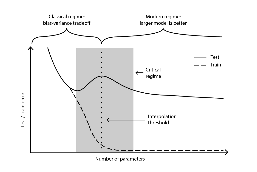
図4. ディープ・ダブルディセント.
Figure 4 illustrates the two successive regimes described above. The first regime is the classic bias-variance tradeoff that seemingly comes with an “optimal” number of parameters. Yet, this minima turns out to be a local minima. There is a second regime, observable if one keeps increasing the number of parameters, that exhibits an asymptotic convergence towards an actual optimal test error for the model.
The deep double descent not only reconciled the statistical and deep learning perspectives, but also demonstrated that generalization remains relatively little understood. It proved that the widely-held theories – commonplace until the late 2010s - presented a distorted perspective on generalization. However, the deep double descent does not yet provide a framework – or something equivalent – that would predict the generalization powers (or lack thereof) of models based on their structure. To date, the approach remains resolutely empirical.
The supply chain thorns
As covered in depth, generalization is exceedingly challenging, and supply chains manage to throw in their own lot of quirks, further intensifying the situation. First, the data supply chain practitioners seek may forever remain inaccessible; not fractionally unseen, but wholly unobservable. Second, the very act of prediction may alter the future, and the validity of the prediction, as decisions are built upon those very predictions. Thus, when approaching generalization in a supply chain context, a two-legged approach should be used; one leg being the statistical soundness of the model and the other being the high-level reasoning that supports the model.
Furthermore, the available data is not always the desired data. Consider a manufacturer that wants to forecast demand in order to decide the quantities to be produced. There is no such thing as historical “demand” data. Instead, the historical sales data represents the best proxy available to the manufacturer to reflect historical demand. However, historical sales are distorted by past stock-outs. Zero sales, as caused by stock-outs, should not be confused with zero demand. While a model can be crafted to rectify this sales history into some sort of demand history, the generalization error of this model is elusive by design, as neither the past nor the future holds this data. In short, “demand” is a necessary but intangible construct.
In machine learning jargon, modeling demand is an unsupervised learning problem where the output of the model is never observed directly. This unsupervised aspect defeats most learning algorithms, and most model validation techniques as well – at least, in their “naïve” flavor. Moreover, it also defeats the very idea of prediction competition, here meaning a simple two-stage process where an original dataset is split into a public (training) subset and a private (validation) subset. The validation itself becomes a modelling exercise, by necessity.
Simply put, the prediction created by the manufacturer will shape, one way or another, the future the manufacturer experiences. A high projected demand means that the manufacturer will ramp up production. If the business is well-run, economies of scale are likely to be achieved in the manufacturing process, hence lowering production costs. In turn, the manufacturer is likely to take advantage of these newfound economics in order to lower prices, hence gaining a competitive edge over rivals. The market, seeking the lowest priced option, may swiftly adopt this manufacturer as its most competitive option, hence triggering a surge of demand well beyond the initial projection.
This phenomenon is known as a self-fulfilling prophecy, a prediction that tends to become true by virtue of the influencing belief that the participants have in the prediction itself. An unorthodox, but not entirely unreasonable, perspective would characterize supply chains as giant self-fulfilling Rube Goldberg contraptions. At a methodological level, this entanglement of observer and observation further complicates the situation, as generalization becomes associated with the capture of the strategic intent that underlies the supply chain developments.
At this point, the generalization challenge, as it presents itself in supply chain, might appear insurmountable. Spreadsheets, which remain ubiquitous in supply chains, certainly hint that this is the default, albeit implicit, position of most companies. A spreadsheet is, however, first and foremost a tool for deferring the resolution of the problem to some ad-hoc human judgement, rather than the application of any systematic method.
Though deferring to human judgement is invariably the incorrect response (in and of itself), it is not a satisfying answer to the problem, either. The presence of stock-outs does not mean that anything goes as far as demand is concerned. Certainly, if the manufacturer has maintained average service levels above 90% during the last three years, it would be highly improbable that (observed) demand could have been 10 times more than sales. Thus, it is reasonable to expect that a systematic method can be engineered to cope with such distortions. Similarly, the self-fulfilling prophecy can be modeled as well, most notably through the notion of policy as understood by the control theory.
Thus, when considering a real-world supply chain, generalization requires a two-legged approach. First, the model must be statistically sound, to the extent permitted by the broad “learning” sciences. This encompasses not only theoretical perspectives like classical statistics and statistical learning, but also empirical endeavors like machine learning and prediction competitions. Reverting to 19th century statistics is not a reasonable proposition for a 21st century supply chain practice.
第二に、モデルは高度な推論によって支えられていなければならない。つまり、モデルのすべての構成要素とモデリングプロセスの各ステップには、サプライチェーンの視点から意味のある正当性が求められる。この要素が欠ければ、通常はサプライチェーン自体の進化、運用エコシステム、またはその下にあるアプリケーション環境のいずれかによって引き起こされる運用上の混乱19がほぼ確実に発生する。実際、高度な推論の本質は、一度だけモデルを機能させることではなく、絶えず変化する環境下で_数年にわたって_持続的に機能させることにある。この推論こそが、モデルの設計が現実および/またはビジネス目標と一致しなくなったと判断した際に、モデルを見直す時期であることを決定する、決して秘密ではない要素である。
遠くから見ると、この提案は以前にスプレッドシートに対して行われた批判―困難な作業を捉えどころのない「人間の判断」に委ねるという批判―に対して脆弱に見えるかもしれない。たとえこの提案が依然としてモデルの評価を人間の判断に委ねるとしても、実行は完全自動化を意図している。したがって、日々の運用は完全に自動化されることを目指しており、たとえ数値レシピのさらなる改善のための継続的なエンジニアリング努力がそうでなくとも。
ノート
-
「メモ化」と呼ばれる重要なアルゴリズム技法があり、これは再計算可能な結果をあらかじめ計算された結果で置き換えることで、計算処理を軽減する代わりにメモリを多く使用する。しかし、この技法は本議論には関係がない。 ↩︎
-
Why Most Published Research Findings Are False, John P. A. Ioannidis, 2005年8月 ↩︎
-
時系列予測の観点から、一般化という概念は「精度」という概念を通じて捉えられる。精度は、時系列を考慮する際の「一般化」の特別なケースと見なすことができる。 ↩︎
-
Makridakis, S.; Andersen, A.; Carbone, R.; Fildes, R.; Hibon, M.; Lewandowski, R.; Newton, J.; Parzen, E.; Winkler, R. (1982年4月). “The accuracy of extrapolation (time series) methods: Results of a forecasting competition”. Journal of Forecasting. 1 (2): 111–153. doi:10.1002/for.3980010202. ↩︎
-
Kaggle in Numbers, Carl McBride Ellis, 2023年2月8日取得, ↩︎
-
1935年の抜粋 “Perhaps we are old fashioned but to us a six-variate analysis based on thirteen observations seems rather like overfitting”(おそらく我々は古風かもしれないが、私たちにとっては13の観測値に基づく6変量解析は過剰適合に思える)は、“The Quarterly Review of Biology” (1935年9月、Volume 10, Number 3, pp. 341–377)に掲載されており、当時すでに統計学における過剰適合の概念が確立されていたことを示唆している。 ↩︎
-
Grenander, Ulf. 『確率過程の経験的スペクトル解析について』. Ark. Mat., 1(6):503–531, 1952年8月. ↩︎
-
Whittle, P. 『時系列におけるフィットテスト』, Vol. 39, No. 3/4 (1952年12月), pp. 309-318 (10ページ), Oxford University Press ↩︎
-
Everitt B.S., Skrondal A. (2010), 『ケンブリッジ統計学辞典』, Cambridge University Press. ↩︎
-
k-分割交差検証においてより大きなkの値を用いることの非漸近的な利点は、中心極限定理から推測できる。この洞察は、kを増加させることで、そもそもk分割法がもたらす改善可能性の全体に対して、約1 / sqrt(k)に近づけることができることを示唆している。 ↩︎
-
サポートベクターネットワーク, Corinna Cortes, Vladimir Vapnik, Machine Learning, 巻20, pp. 273–297 (1995) ↩︎
-
Vapnik–Chervonenkis (VC) 理論は、「学習」とは何かを形式化するための唯一の候補ではなかった。Valiantの1984年のPAC(Probably Approximately Correct)フレームワークは、形式的な学習アプローチへの道を切り開いた。しかし、PACフレームワークは、ミレニアム期にVC理論が享受した大きな支持と運用上の成功を欠いていた。 ↩︎
-
ランダムフォレスト, Leo Breiman, Machine Learning, 巻45, pp. 5–32 (2001) ↩︎
-
数学理論に大きく触発されたサポートベクターマシン(SVM)の不運な結果の一つは、これらのモデルが現代のコンピュータハードウェアに対してほとんど「機械的親和性」を持たないことである。何百万もの観測値を含む大規模データセットの処理において、代替手段と比較してSVMが相対的に不十分であったことが、これらの手法の衰退を招いた。 ↩︎
-
XGBoostとLightGBMは、機械学習界で広く人気のあるアンサンブル手法の2つのオープンソース実装である。 ↩︎
-
簡潔さのために、ここではやや単純化している。統計モデルの「正則化」に専念する研究分野が存在する。正則化制約下では、古典的なモデルである線形回帰でさえも、パラメータの数が観測値の数を安全に超える場合がある。正則化が存在すると、各パラメータ値はもはや完全な自由度を表すのではなく、その一部に過ぎない。したがって、パラメータの数ではなく、自由度の数を参照する方が適切である。これらの周辺的な考察がここで提示する見解の本質を根本的に変えるものではないため、単純化したバージョンで十分である。 ↩︎
-
実際、因果関係は逆である。ディープラーニングの先駆者たちは、元々のモデル―ニューラルネットワーク―をほぼ線形代数学に依存するより単純なモデルへと再設計することに成功した。この再設計の目的は、汎用性よりも生の計算能力、すなわちGPUに重きを置くコンピュータハードウェア上でこれらの新しいモデルを動作させることを可能にするためであった。 ↩︎
-
Deep Double Descent: Where Bigger Models and More Data Hurt, Preetum Nakkiran, Gal Kaplun, Yamini Bansal, Tristan Yang, Boaz Barak, Ilya Sutskever, 2019年12月 ↩︎
-
サプライチェーンにおけるデータサイエンスの取り組みの大部分は失敗に終わる。私のざっくりとした観察では、サプライチェーンの仕組みを理解していないデータサイエンティストの無知が、これらの失敗の根本原因であることが多いと示唆している。新たに訓練されたデータサイエンティストにとって、最新かつ最も輝かしいオープンソースの機械学習パッケージを活用するのは非常に魅力的であるが、すべてのモデリング技術が高度な推論を支えるのに同等に適しているわけではない。実際、「主流」の技術の多くは、ホワイトボックス化プロセスにおいては実にひどいものである。 ↩︎